Planar
Maps
in
4
bits/edge | | http://arxiv.org/abs/math/0104147
Last
revised:
22nd December 2001 |
| Fred
Curtis,
Dept.
Inapplicable
Mathematics,
Miskatonic
University,
Arkham,
MA
65261. | |
|
Abstract:
Existing
planar
map
encodings
neglect
maps
with
loops.
The
presented
scheme
encodes
any
connected
planar
map
in
4
bits/edge.
Encoding
and
decoding
time
is
O(edges). |
|
|
| In
this
paper
graph
has
the
most
general
sense,
admitting
loops
and
multiple
edges.
Graphs
discussed
here
are
assumed
connected,
unlabelled,
undirected,
and
finite.
A
map
is
an
embedding
of
a
graph
in
the
open
plane;
an
embedding
in
the
sphere
is
trivially
viewed
as
a
map. |
| Existing
map
encodings
neglect
maps
with
loops.
[Turán84]
encodes
maps
without
loops
or
multiple
edges
in
asymptotically
4
bits/edge
.
[Keeler95]
encodes
maps
without
loops
or
degree-1
vertices
in
3
bits/edge.
Shorter
encodings
exist
[Chuang98]
for
even
more
specialised
graphs. |
| The
scheme
below
encodes
any
map
in
4
bits/edge
and
requires
an
(unrestricted)
choice
of
spanning
tree
and
directed
root
edge.
Decoding
recovers
the
map,
spanning
tree
and
root
edge. |
|
Map
edges
are
undirected;
'directed
edge'
means
a
pair
composed
of
a
map
edge
and
a
direction.
'CW'
means
'clockwise';
'CCW'
means
'counter-clockwise'.
The
empty
map
is
encoded
as
the
empty
bit
string.
A
map
M
with
m > 0
edges
is
encoded
as
follows: |
| 1. | Choose
a
directed
edge
eM
as
the
root
edge
of
M. |
| 2. | Choose
a
spanning
tree
S
of
M.
An
edge
of
M
is
a
tree
edge
if
it
lies
in
S,
a
non-tree
edge
if
not. |
| 3. | Make
a
tree
map
T
from
M
by
splitting
each
non-tree
edge
e
in
M
into
two
labelled
leaf
edges;
label
with
"["
(resp.
"]")
the
new
edge
in
T
corresponding
to
the
initial
(resp.
final)
segment
of
e
tracing
CCW
about
the
circuit
made
by
e
and
elements
of
S.
If
eM
is
a
tree
edge
then
the
directed
root
edge
eT
of
T
is
the
corresponding
edge
in
T,
otherwise
eT
is
the
directed
labelled
leaf
edge
corresponding
to
the
directed
initial
segment
of
eM.
Fig.
1
shows
examples. |
| 4. | Treat
T
as
a
degenerate
boundary
of
the
open
plane
in
which
each
edge
occurs
twice.
List
T's
edges
in
CW
order
as
viewed
from
a
point
in
the
plane,
starting
with
the
CW
aspect
of
eT.
The
first
occurrence
of
an
unlabelled
edge
is
encoded
"(";
the
second
is
encoded
")";
the
first
occurrence
of
a
labelled
leaf
edge
is
encoded
with
the
edge's
label. |
| |
Fig.
1:
Two
encodings
of
a
map
M
with
the
same
choice
of
S
but
different
eM
Solid
(dotted)
lines
are
tree
(non-tree)
edges
in
M,
unlabelled
(labelled)
edges
in
T. | 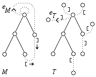 | | 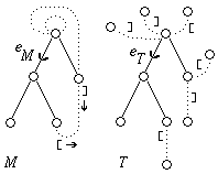 | | (a)
Encoding:
] ( ( ) ( [ ) ) ( ] [ ) [ ] | | (b)
Encoding:
( ( ) ( [ ) ) ( ] [ ) [ ] ] |
|
Each
edge
of
M
encodes
a
pair
of
symbols,
so
the
encoding
is
a
string
of
length
2m
over
the
alphabet
( ) [ ] ,
requiring
4m
bits,
or
4
bits/edge.
Terminate
an
encoding
(including
the
encoding
of
the
empty
map)
with
an
additional
unbalanced
)
symbol
to
indicate
end-of-encoding
in
a
symbol
stream
or
other
circumstance
where
the
length
or
end
of
the
encoding
is
not
apparent.
T
is
recovered
from
an
encoded
string
as
follows:
| 1. | Create
an
empty
(tree)
map
T
with
a
single
vertex.
Set
the
marker
v
to
refer
to
this
vertex. |
| 2. | For
each
successive
symbol
s
in
the
encoding,| - | If
s
is
"("
then
add
an
unlabelled
leaf
edge
to
T
at
v
following
CCW
about
v
from
any
edges
previously
attached
to
v.
Set
v
to
refer
to
the
newly
created
leaf
vertex. | | - | If
s
is
")"
then
set
v
to
refer
to
the
parent
vertex
of
v. | | - | If
s
is
"["
or
"]"
then
add
a
labelled
leaf
edge
to
T
at
v
following
CCW
about
v
from
any
edges
previously
attached
to
v.
Leave
v
unchanged. |
|
| 3. | A
subtree
TS
of
T
is
formed
by
the
initial
vertex,
unlabelled
edges
and
their
endpoints.
eT
is
the
first
edge
added
to
T,
directed
away
from
the
initial
vertex. |
The
labelled
leaf
edges
of
T
can
be
joined
in
pairs
to
form
a
map
J
such
that
the
initial
(resp.
final)
segment
of
each
joined
edge
in
J
corresponds
to
a
leaf
labelled
"["
(resp.
"]")
in
T
when
traversing
CCW
the
circuit
formed
in
J
by
the
joined
edge
and
TS.
The
original
map
M
is
an
example
of
such
a
map
J,
and
the
only
example
since
J
is
uniquely
determined
by
its
pairing
of
labelled
edges
and
there
is
only
one
pairing:
suppose
edges
e[a, ... e]y, ... e]z
occur
in
CCW
order
about
TS
and
e[a
may
be
paired
with
e]y
(resp.
e]z)
in
map
J1
(resp.
J2).
In
J2,
e[a
is
matched
with
e]z
so
e]y
must
be
matched
with
some
edge
e[b
between
e[a
and
e]y.
Similar
reasoning
with
the
edge
sequence
e[a, ... e[b, ... e]y
in
J1
leads
to
an
infinite
regression.
M
is
recovered
from
T
by
constructing
the
unique
map
J
above.
The
spanning
tree
S
of
M
is
the
tree
corresponding
to
TS.
If
eT
is
unlabelled,
eM
is
the
corresponding
directed
edge
in
M;
otherwise,
eM
is
the
directed
joined
edge
in
M
with
a
directed
initial
segment
corresponding
to
eT
in
T.
Encoding
and
decoding
times
are
O(m)
given,
e.g.,
the
adjacency
list
representation
of
[Keeler95]
or
the
quad-edge
data
structure
[Guibas85].
In
encoding,
O(m)
time
is
taken
to
choose
S,
traverse
T
emitting
symbols
and
compute
labels
for
T
using
a
copy
of
M
(remove
each
successive
non-tree
edge
e
adjacent
to
the
unbounded
region;
e
CCW
about
the
unbounded
region
opposes
e
CCW
about
the
circuit
made
by
e
and
elements
of
S).
In
decoding,
T
is
created
in
O(m)
time
and
the
labelled
edges
created
in
CCW
order
about
TS
are
joined
in
O(m)
time
as
balanced
parentheses.
Implicit
Vertex,
Edge
and
Face
Orderings
Implicit
orderings
are
useful
when
encoding
auxilliary
map
data,
e.g.,
a
connected
signed
planar
map
(representing,
e.g.,
a
link
diagram
in
knot
theory)
has
a
+/-
sign
on
each
edge,
and
may
be
encoded
in
5
bits/edge
by
appending
sign
bits
(in
an
implicit
edge
order)
to
the
map
encoding.
Examples
of
implicit
orderings
are:
Vertex
ordering:
order
map
vertices
by
in-order
traversal
of
the
spanning
tree
S.
Edge
ordering:
each
symbol
in
the
map
encoding
corresponds
to
a
map
edge;
order
map
edges
by
first
occurrence
of
a
matching
symbol
within
the
map
encoding.
Face
ordering:
assign
each
map
edge
a
direction
-
that
of
the
matching
"["-labelled
or
unlabelled
edge
in
the
tree
T,
directed
away
from
the
origin
vertex
of
eT.
Associate
with
each
directed
map
edge
e
an
ordered
face-pair
(f1, f2)
where
e
appears
CCW
(resp.
CW)
in
a
CCW
traversal
of
the
boundary
of
f1
(resp.
f2).
Order
map
faces
by
first
occurence
in
a
concatenated
list
(in
an
implicit
edge
order)
of
face-pairs.
Canonical
Encodings
A
canonical
encoding
of
a
map
may
be
obtained
by
considering
all
possible
encodings
and
selecting
some
unique
representative,
e.g.
the
first
in
a
lexically
ordered
list
of
possible
encodings.
The
presented
encoding
scheme
requires
an
arbitrary
choice
of
directed
root
edge
and
spanning
tree,
yielding
a
combinatorially
large
number
of
candidate
encodings.
This
number
is
reduced
by
making
the
spanning
tree
a
function
of
the
directed
root
edge,
e.g.
the
tree
obtained
in
a
depth-first
exploration
of
the
map
starting
from
the
root
edge.
For
graph
embeddings
on
the
sphere
there
is
an
additional
arbitrary
choice
of
some
face
to
serve
as
the
outer
unbounded
region
of
the
plane
in
the
encoding
(the
plane
defines
the
direction
of
the
non-tree
edges
in
the
encoding);
this
choice
may
be
restricted,
e.g.,
to
the
unique
face
where
a
CCW
traversal
of
bounding
edges
encounters
the
CW
aspect
of
the
root
edge.
Thus
the
encoding
for
a
map
or
spherical
embedding
can
be
uniquely
determined
by
the
choice
of
directed
root
edge,
yielding
2m
candidate
encodings
for
a
map
with
m
edges.
Choices
for
candidate
encodings
may
be
further
narrowed
by
considering
some
distinguished
subset
of
edges,
e.g.
only
edges
adjoining
faces
or
vertices
of
minimal
degree,
but
possibilities
are
limited
for
relatively
featureless
maps
with
high
symmetry.
O(m2)
time
and
O(m)
space
are
taken
by
considering
all
2m
candidate
encodings.
Canonical
encodings
have
wider
application
in
grouping
maps
into
equivalence
classes:
those
described
above
group
maps
by
isomorphism
(isotopy
within
the
oriented
plane
or
sphere);
other
canonical
encodings
may
group
maps
by,
e.g.,
ignoring
orientation
and
considering
a
map
and
its
mirror
image
as
equivalent.
References
| [Chuang98] | Richie
Chih-Nan
Chuang
&
Ashim
Garg
&
Xin
He
&
Ming-Yang
Kao
&
Hsueh-I
Lu.
Compact
Encodings
of
Planar
Graphs
via
Canonical
Orderings
and
Multiple
Parentheses.
Springer-Verlag
Lecture
Notes
in
Computer
Science 1443,
pp. 118-129.
Document
downloadable
at
[http://citeseer.nj.nec.com/chuang98compact.html] |
| [Guibas85] | Leonidas
Guibas
&
Jorge
Stolfi.
Primitives
for
the
Manipulation
of
General
Subdivisions
and
the
Computation
of
Voronoi
Diagrams.
ACM
Transactions
on
Graphics,
vol 4,
no 2,
April 1985,
pp 74-123. |
| [Keeler95] | Kenneth
Keeler
&
Jeffery
Westbrook.
Short
Encodings
of
Planar
Graphs
and
Maps.
Discrete
Applied
Mathematics,
vol 58
(1995),
pp. 239-252.
Document
downloadable
at
[http://citeseer.nj.nec.com/keeler95short.html] |
| [Turán84] | György
Turán.
On
the
succinct
representation
of
graphs.
Discrete
Applied
Mathematics,
vol 8
(1984),
pp. 289-294. |
Revision
History
- 15th
April,
2001
-
Initial
revision
giving
encoding
scheme.
- 22nd
December,
2001
-
Added
notes
on
implicit
orderings,
canonical
forms
and
terminating
symbol
for
symbol
streams.